From Paper to Code: Understanding and Reproducing “Implicit Neural Representations with Periodic Activation Functions”

From Paper to Code: Understanding and Reproducing “Implicit Neural Representations with Periodic Activation Functions”#

Code: GitHub Repository https://vsitzmann.github.io/siren/ Source Code in My Repo: ../../../../code/NeRF/siren-master/explore_siren.ipynb

Paper Reading Notes#

1. Highlights#

This paper proposes SIREN, a novel method that uses continuous coordinates as input instead of discrete meshes to represent images, enabling arbitrary-resolution sampling and super-resolution image reconstruction.

For example, traditional meshes can only retrieve colors at integer coordinates, whereas SIREN allows querying at any real-valued coordinate such as (3.45, 4.98).

SIREN based on periodic activation functions, along with a principled initialization scheme to ensure stable training of deep networks. They demonstrate high-fidelity representations across images, videos, audio, and 3D shapes, and further show that SIRENs can solve partial differential equations (PDEs) directly from derivative supervision. In addition, they combine SIRENs with hypernetworks to learn priors over implicit function spaces, enabling tasks such as sparse image inpainting.

2. Background#

How to represent a signal is a fundamental question across science and engineering.
Traditional representations are typically discrete, such as pixel grids for images or voxel grids for 3D shapes.
However, these discrete formats suffer from issues like high memory usage, limited resolution, and difficulty in computing derivatives.

Recently, implicit neural representations (INRs) have emerged as a powerful alternative.
Instead of storing signals explicitly, they use neural networks to map coordinates $x$ (e.g., spatial or spatiotemporal) directly to signal values $\Phi(x)$.

For example, in many physical problems, we aim to learn a function $\Phi$ that satisfies:

\[ F(x, \Phi(x), \nabla_x \Phi(x), \nabla^2_x \Phi(x), \ldots) = 0 \tag{1} \]

This includes problems in physics, imaging, graphics, and differential equations.

Most existing INR methods are built on ReLU-based MLPs. While these can fit low-frequency components, they struggle with high-frequency signals and fail to represent higher-order derivatives well — which are essential for many physical systems.

3. Method Overview#

This paper introduces SIREN (Sinusoidal Representation Networks), a neural network architecture that uses the sine function as its activation:

\[ \phi_i(x_i) = \sin(W_i x_i + b_i) \]

A full SIREN network is:

\[ \Phi(x) = W_n \cdot (\phi_{n-1} \circ \phi_{n-2} \circ \cdots \circ \phi_0)(x) + b_n \tag{4} \]

The key advantage is that any derivative of a sine is also a sine or cosine, which preserves expressiveness through derivatives.
This makes SIREN particularly powerful for modeling natural signals and their derivatives — such as gradients and Laplacians.

They define a general optimization objective to solve constraint problems of the form: $$ \begin{aligned} & \text{Find } \Phi(x) \text{ such that} \\ & C_m\left(a(x), \Phi(x), \nabla \Phi(x), \ldots\right) = 0, \\ & \forall x \in \Omega_m,\quad m=1,\ldots,M \end{aligned} $$

The corresponding loss function is:

\[ \mathcal{L} = \int_\Omega \sum_{m=1}^M \mathbf{1}_{\Omega_m}(x) \left\| C_m(a(x), \Phi(x), \nabla \Phi(x), \ldots) \right\| dx \tag{3} \]

The authors further propose a principled initialization scheme for SIREN:

Weights $W_i$ are sampled from $U\left(-\sqrt{\frac{6}{n}}, \sqrt{\frac{6}{n}}\right)$
The first layer uses a higher frequency $\omega_0 = 30$ to match the spectrum of natural signals

This ensures stability in training and allows SIRENs to scale deeper without vanishing or exploding gradients.

4. References#

Vincent Sitzmann et al., Implicit Neural Representations with Periodic Activation Functions, arXiv:2006.09661, 2020
Ben Mildenhall et al., NeRF: Representing Scenes as Neural Radiance Fields for View Synthesis, arXiv:2003.08934
Jeong Joon Park et al., DeepSDF, CVPR 2019
Maziar Raissi et al., Physics-informed Neural Networks, JCP 2019
David Ha et al., Hypernetworks, ICLR 2017

Code Reproduction with Explanation: SIREN in Action – Image, Audio, and PDE Solving#

This implementation is based on the streamlined version of SIREN provided in the official Colab notebook: Implicit Neural Activations with Periodic Activation Functions.

Make sure that you have enabled the GPU under Edit -> Notebook Settings!

We will then reproduce the following results from the paper:

Fitting an image
Fitting an audio signal
Solving Poisson’s equation
Initialization scheme & distribution of activations
Distribution of activations is shift-invariant

We will also explore Siren’s behavior outside of the training range.

Let’s go! First, some imports, and a function to quickly generate coordinate grids.

import torch
from torch import nn
import torch.nn.functional as F
from torch.utils.data import DataLoader, Dataset
import os

from PIL import Image
from torchvision.transforms import Resize, Compose, ToTensor, Normalize
import numpy as np
import skimage
import matplotlib.pyplot as plt

import time

def get_mgrid(sidelen, dim=2):
    '''Generates a flattened grid of (x,y,...) coordinates in a range of -1 to 1.
    sidelen: int
    dim: int'''
    tensors = tuple(dim * [torch.linspace(-1, 1, steps=sidelen)])
    mgrid = torch.stack(torch.meshgrid(*tensors), dim=-1)
    mgrid = mgrid.reshape(-1, dim)
    return mgrid

Now, we code up the sine layer, which will be the basic building block of SIREN. This is a much more concise implementation than the one in the main code, as here, we aren’t concerned with the baseline comparisons.

class SineLayer(nn.Module):
    # See paper sec. 3.2, final paragraph, and supplement Sec. 1.5 for discussion of omega_0.
    
    # If is_first=True, omega_0 is a frequency factor which simply multiplies the activations before the 
    # nonlinearity. Different signals may require different omega_0 in the first layer - this is a 
    # hyperparameter.
    
    # If is_first=False, then the weights will be divided by omega_0 so as to keep the magnitude of 
    # activations constant, but boost gradients to the weight matrix (see supplement Sec. 1.5)
    
    def __init__(self, in_features, out_features, bias=True,
                 is_first=False, omega_0=30):
        super().__init__()
        self.omega_0 = omega_0
        self.is_first = is_first
        
        self.in_features = in_features
        self.linear = nn.Linear(in_features, out_features, bias=bias)
        
        self.init_weights()
    
    def init_weights(self):
        with torch.no_grad():
            if self.is_first:
                self.linear.weight.uniform_(-1 / self.in_features, 
                                             1 / self.in_features)      
            else:
                self.linear.weight.uniform_(-np.sqrt(6 / self.in_features) / self.omega_0, 
                                             np.sqrt(6 / self.in_features) / self.omega_0)
        
    def forward(self, input):
        return torch.sin(self.omega_0 * self.linear(input))
    
    def forward_with_intermediate(self, input): 
        # For visualization of activation distributions
        intermediate = self.omega_0 * self.linear(input)
        return torch.sin(intermediate), intermediate
    
    

And finally, differential operators that allow us to leverage autograd to compute gradients, the laplacian, etc.

def laplace(y, x):
    grad = gradient(y, x)
    return divergence(grad, x)


def divergence(y, x):
    div = 0.
    for i in range(y.shape[-1]):
        div += torch.autograd.grad(y[..., i], x, torch.ones_like(y[..., i]), create_graph=True)[0][..., i:i+1]
    return div


def gradient(y, x, grad_outputs=None):
    if grad_outputs is None:
        grad_outputs = torch.ones_like(y)
    grad = torch.autograd.grad(y, [x], grad_outputs=grad_outputs, create_graph=True)[0]
    return grad

Experiments#

For the image fitting and poisson experiments, we’ll use the classic cameraman image.

def get_cameraman_tensor(sidelength):
    img = Image.fromarray(skimage.data.camera())        
    transform = Compose([
        Resize(sidelength),
        ToTensor(),
        Normalize(torch.Tensor([0.5]), torch.Tensor([0.5]))
    ])
    img = transform(img)
    return img

For a 256×256 image, each pixel corresponds to a 2D coordinate, so the input coords has shape $(1, 65536, 2)$. After passing through the network, the output shape becomes $(1, 65536, 1)$, representing the predicted signal (e.g., color or intensity) at each coordinate.

In each SineLayer, the input first goes through a linear transformation and is then scaled by $\omega_0$ before applying the sine activation. The $\omega_0$ controls the frequency of the sine function: a larger $\omega_0$ enables the network to capture higher-frequency details in the data.

Notes on Input Coordinates, Omega, and Activation#

In each SineLayer, the activation is defined as torch.sin(self.omega_0 * self.linear(input)). The input coords are sampled from $[-1, 1]$. The frequency factor $\omega_0$ scales the output of the linear layer before applying the sine function:

A larger $\omega_0$ amplifies the pre-activation values, meaning a small change in the input coordinate leads to a large change in the sine input, resulting in rapid oscillations. This makes the network highly sensitive to fine, high-frequency features.
A smaller $\omega_0$ causes smoother oscillations, favoring the modeling of low-frequency, slowly varying structures.

Here, torch.sin serves as the activation function, introducing periodic nonlinearity after each linear transformation.

class Siren(nn.Module):
    def __init__(self, in_features, hidden_features, hidden_layers, out_features, outermost_linear=False, 
                 first_omega_0=30, hidden_omega_0=30.):
        super().__init__()
        
        self.net = []
        self.net.append(SineLayer(in_features, hidden_features, 
                                  is_first=True, omega_0=first_omega_0))

        for i in range(hidden_layers):
            self.net.append(SineLayer(hidden_features, hidden_features, 
                                      is_first=False, omega_0=hidden_omega_0))

        if outermost_linear:
            final_linear = nn.Linear(hidden_features, out_features)
            
            with torch.no_grad():
                final_linear.weight.uniform_(-np.sqrt(6 / hidden_features) / hidden_omega_0, 
                                              np.sqrt(6 / hidden_features) / hidden_omega_0)
                
            self.net.append(final_linear)
        else:
            self.net.append(SineLayer(hidden_features, out_features, 
                                      is_first=False, omega_0=hidden_omega_0))
        
        self.net = nn.Sequential(*self.net)
    
    def forward(self, coords):
        coords = coords.clone().detach().requires_grad_(True) # allows to take derivative w.r.t. input
        output = self.net(coords)
        return output, coords        

    def forward_with_activations(self, coords, retain_grad=False):
        '''Returns not only model output, but also intermediate activations.
        Only used for visualizing activations later!'''
        activations = OrderedDict()

        activation_count = 0
        x = coords.clone().detach().requires_grad_(True)
        activations['input'] = x
        for i, layer in enumerate(self.net):
            if isinstance(layer, SineLayer):
                x, intermed = layer.forward_with_intermediate(x)
                
                if retain_grad:
                    x.retain_grad()
                    intermed.retain_grad()
                    
                activations['_'.join((str(layer.__class__), "%d" % activation_count))] = intermed
                activation_count += 1
            else: 
                x = layer(x)
                
                if retain_grad:
                    x.retain_grad()
                    
            activations['_'.join((str(layer.__class__), "%d" % activation_count))] = x
            activation_count += 1

        return activations

Fitting an image#

First, let’s simply fit that image!

We seek to parameterize a greyscale image $f(x)$ with pixel coordinates $x$ with a SIREN $\Phi(x)$.

That is we seek the function $\Phi$ such that: $\mathcal{L}=\int_{\Omega} \lVert \Phi(\mathbf{x}) - f(\mathbf{x}) \rVert\mathrm{d}\mathbf{x}$ is minimized, in which $\Omega$ is the domain of the image.

We write a little datast that does nothing except calculating per-pixel coordinates:

class ImageFitting(Dataset):
    def __init__(self, sidelength):
        super().__init__()
        img = get_cameraman_tensor(sidelength)
        self.pixels = img.permute(1, 2, 0).view(-1, 1)
        self.coords = get_mgrid(sidelength, 2)

    def __len__(self):
        return 1

    def __getitem__(self, idx):    
        if idx > 0: raise IndexError
            
        return self.coords, self.pixels

Let’s instantiate the dataset and our Siren. As pixel coordinates are 2D, the siren has 2 input features, and since the image is grayscale, it has one output channel.

cameraman = ImageFitting(256)
dataloader = DataLoader(cameraman, batch_size=1, pin_memory=True, num_workers=0)

img_siren = Siren(in_features=2, out_features=1, hidden_features=256, 
                  hidden_layers=3, outermost_linear=True)
img_siren.cuda()

/home/xqgao/anaconda3/envs/inr/lib/python3.12/site-packages/torch/functional.py:534: UserWarning: torch.meshgrid: in an upcoming release, it will be required to pass the indexing argument. (Triggered internally at /opt/conda/conda-bld/pytorch_1729647329220/work/aten/src/ATen/native/TensorShape.cpp:3595.)
  return _VF.meshgrid(tensors, kwargs)  # type: ignore[attr-defined]





Siren(
  (net): Sequential(
    (0): SineLayer(
      (linear): Linear(in_features=2, out_features=256, bias=True)
    )
    (1): SineLayer(
      (linear): Linear(in_features=256, out_features=256, bias=True)
    )
    (2): SineLayer(
      (linear): Linear(in_features=256, out_features=256, bias=True)
    )
    (3): SineLayer(
      (linear): Linear(in_features=256, out_features=256, bias=True)
    )
    (4): Linear(in_features=256, out_features=1, bias=True)
  )
)

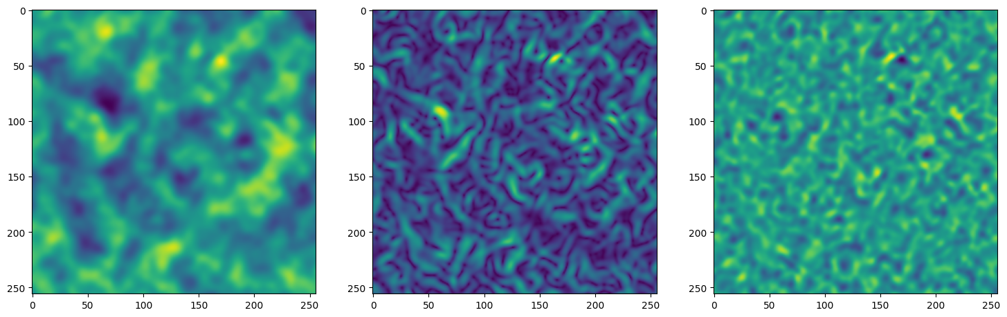
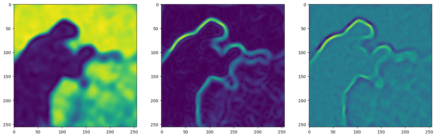
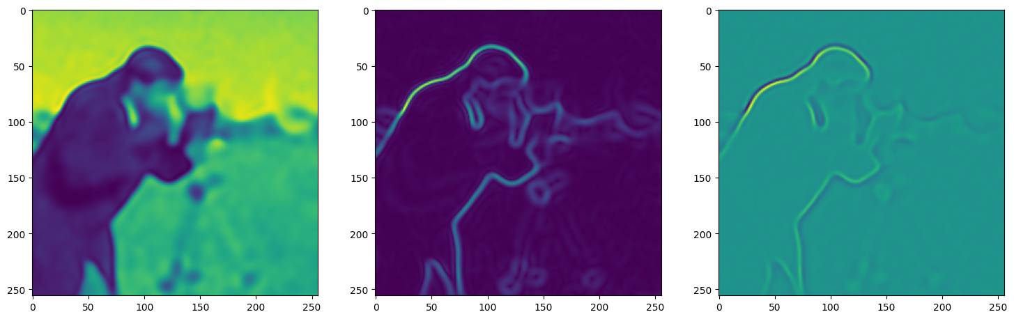
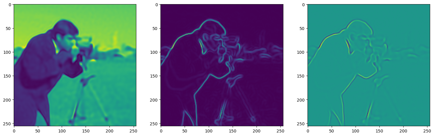
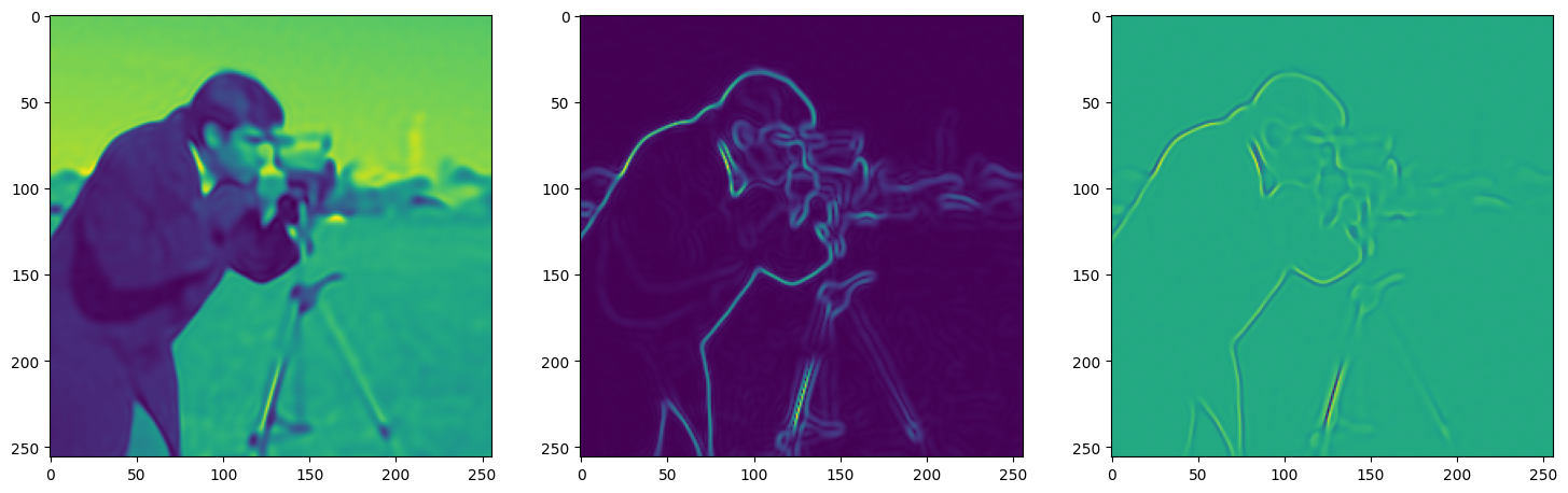
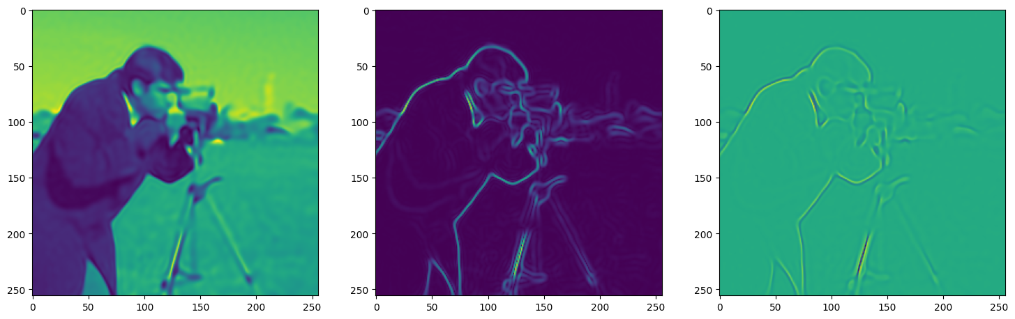
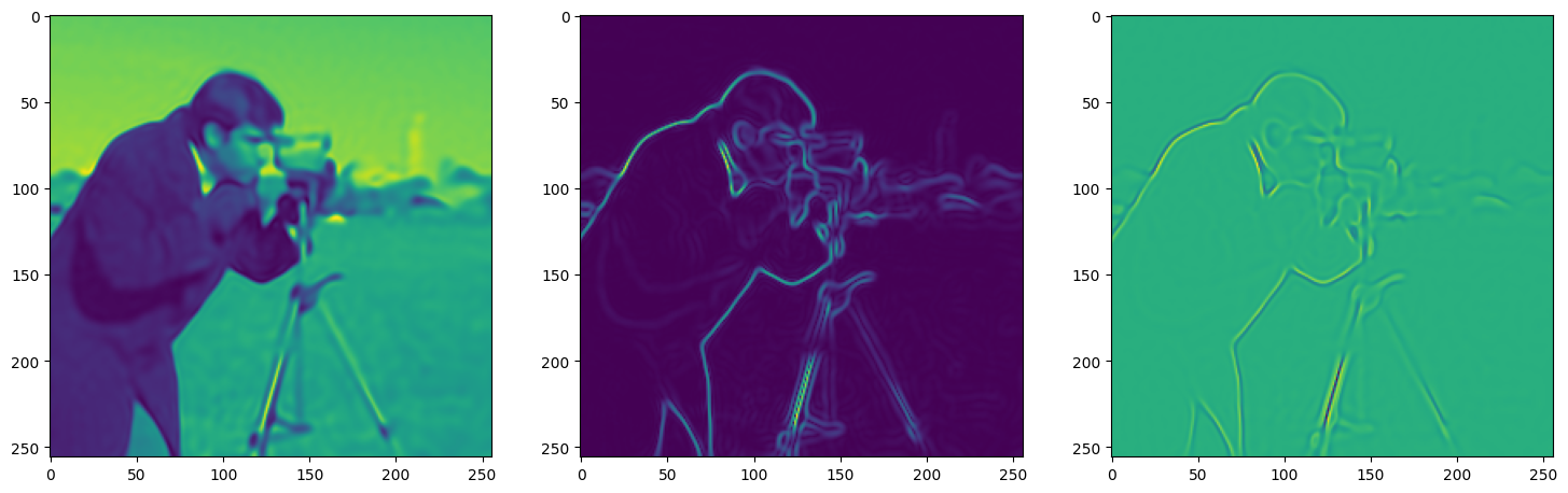
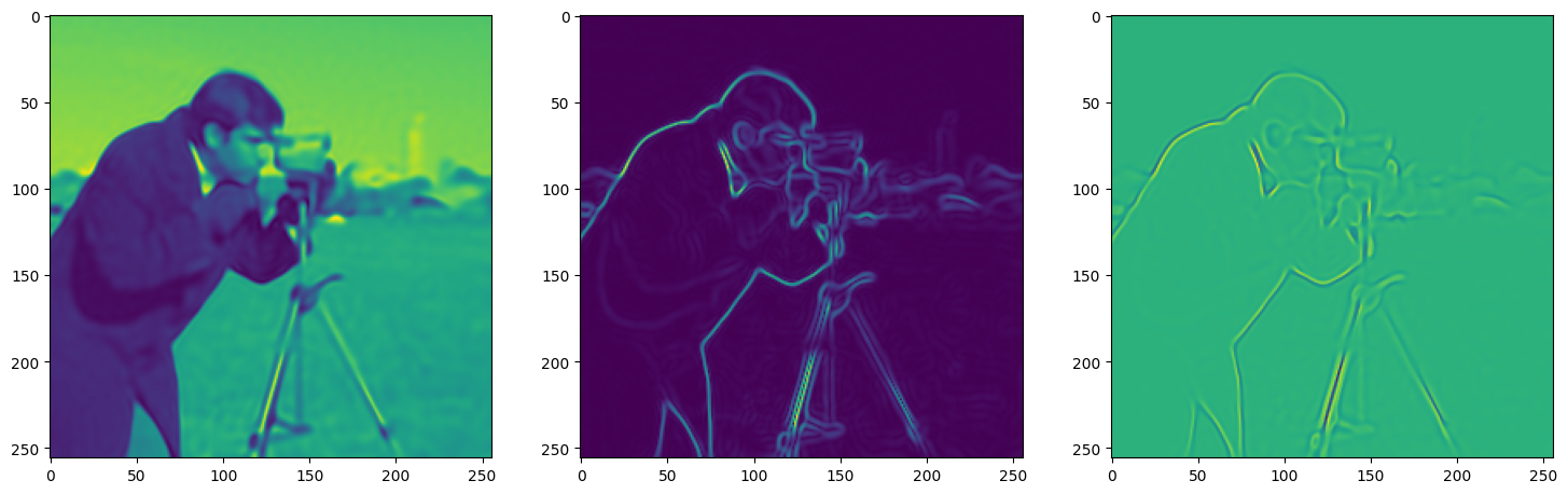
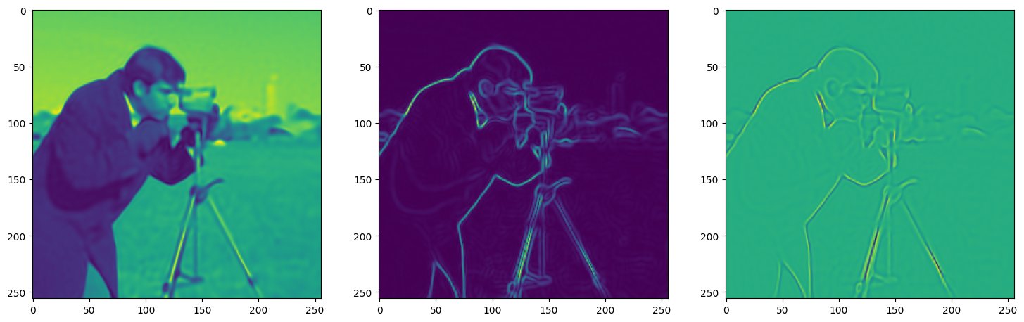
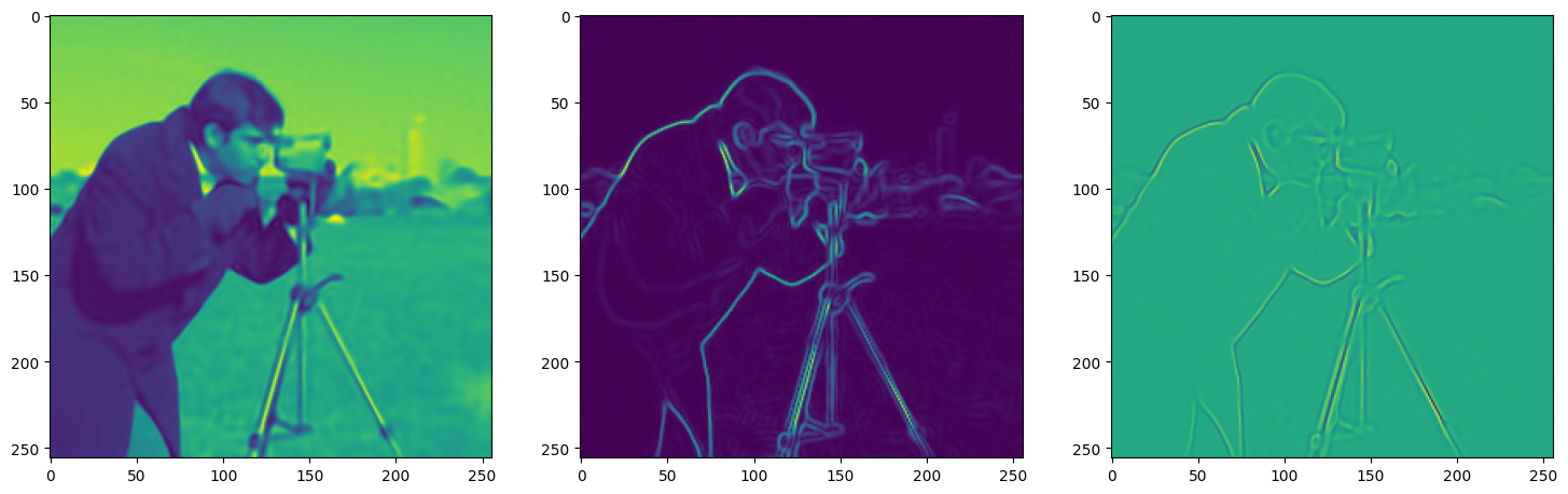
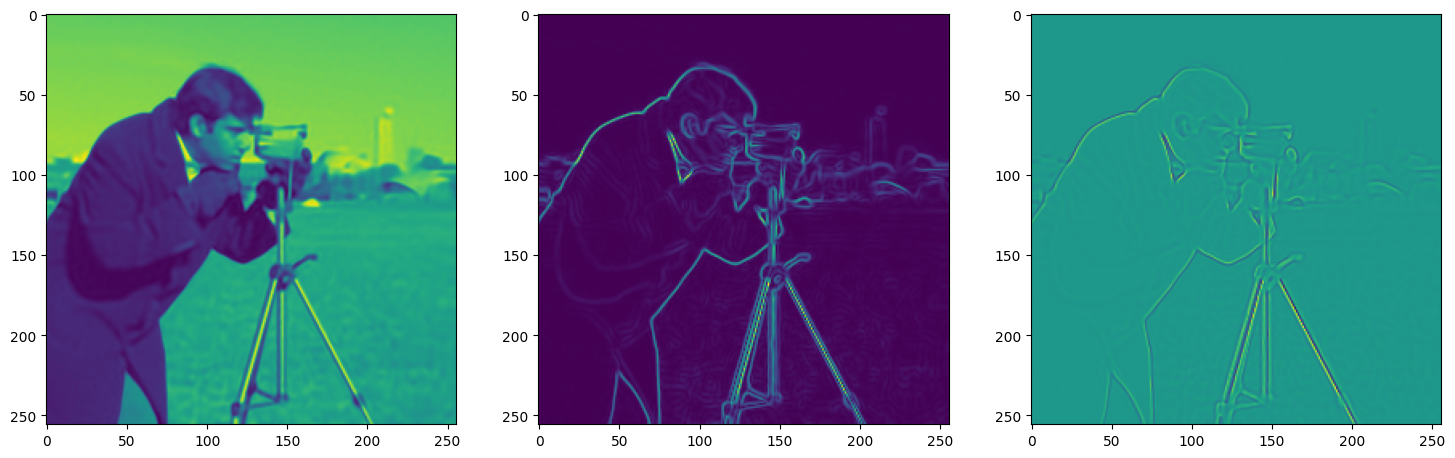
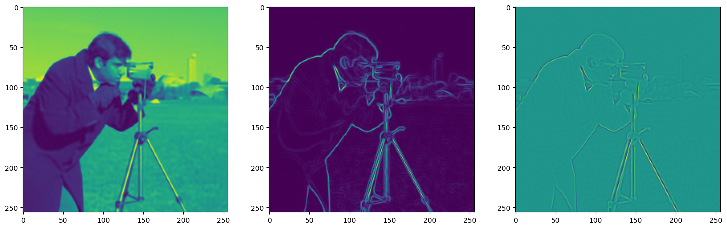
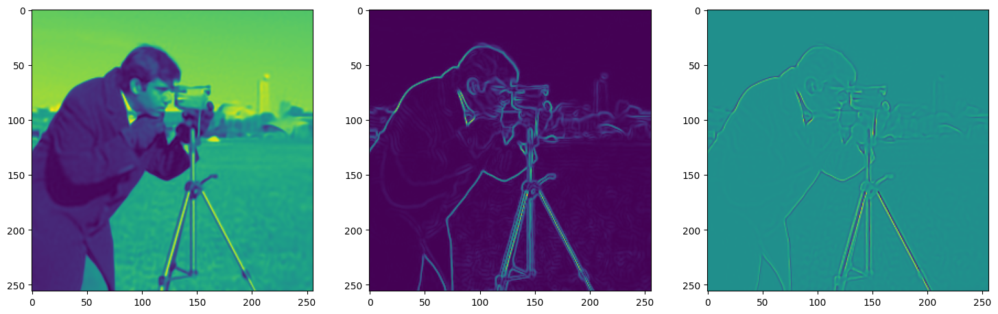
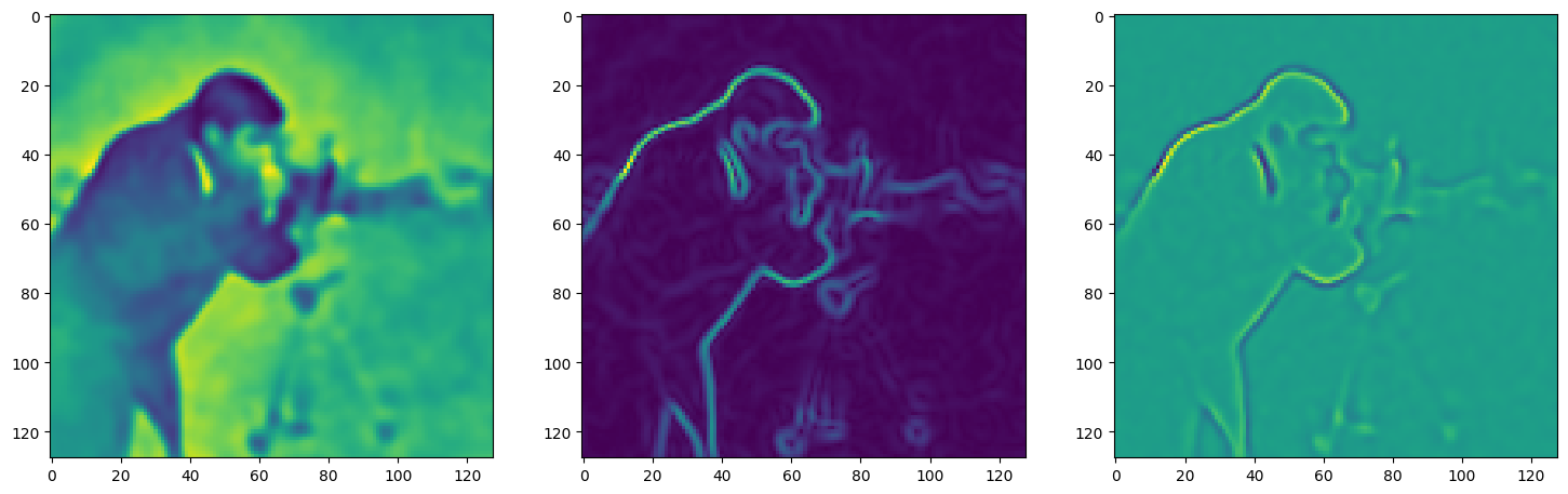
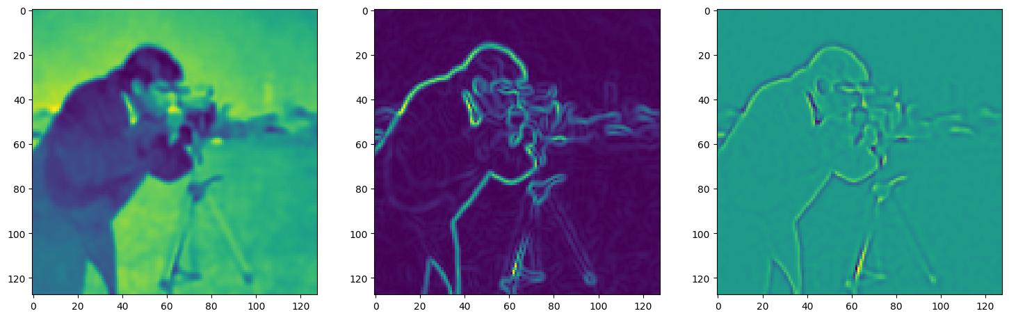
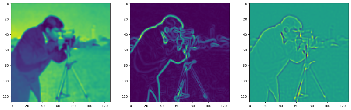
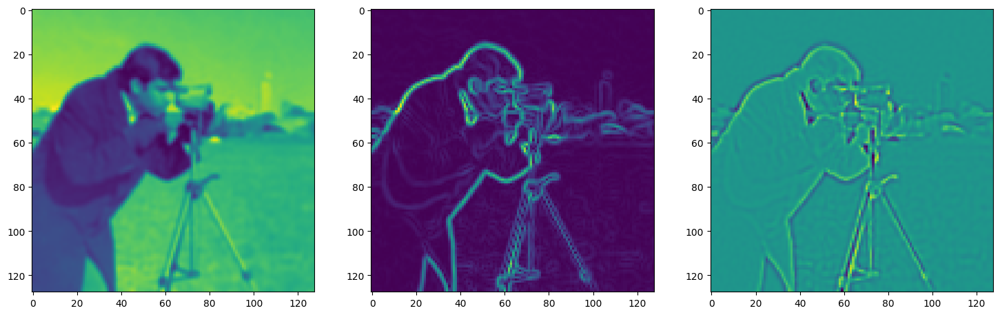
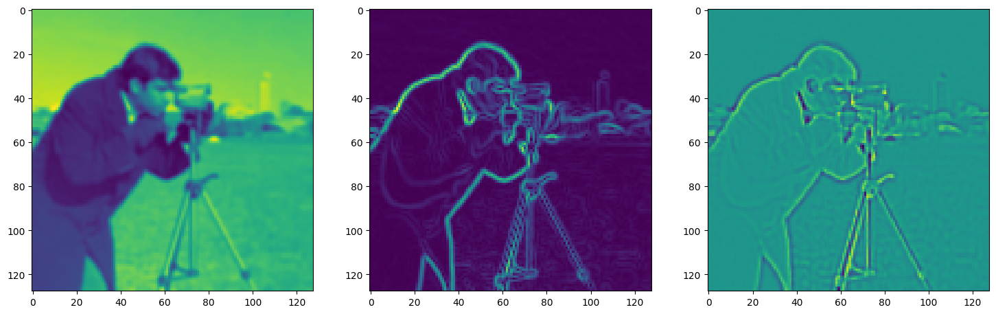
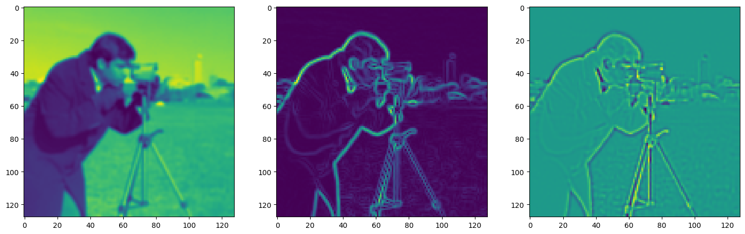
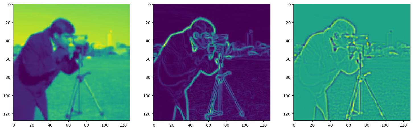
We now fit Siren in a simple training loop. Within only hundreds of iterations, the image and its gradients are approximated well.

total_steps = 500 # Since the whole image is our dataset, this just means 500 gradient descent steps.
steps_til_summary = 10

optim = torch.optim.Adam(lr=1e-4, params=img_siren.parameters())

model_input, ground_truth = next(iter(dataloader))
model_input, ground_truth = model_input.cuda(), ground_truth.cuda()

for step in range(total_steps):
    model_output, coords = img_siren(model_input)    
    loss = ((model_output - ground_truth)2).mean()
    
    if not step % steps_til_summary:
        print("Step %d, Total loss %0.6f" % (step, loss))
        img_grad = gradient(model_output, coords)
        img_laplacian = laplace(model_output, coords)

        fig, axes = plt.subplots(1,3, figsize=(18,6))
        axes[0].imshow(model_output.cpu().view(256,256).detach().numpy())
        axes[1].imshow(img_grad.norm(dim=-1).cpu().view(256,256).detach().numpy())
        axes[2].imshow(img_laplacian.cpu().view(256,256).detach().numpy())
        plt.show()

    optim.zero_grad()
    loss.backward()
    optim.step()

Step 0, Total loss 0.321211

png

Step 10, Total loss 0.052471

png

Step 20, Total loss 0.023199

png

Step 30, Total loss 0.017426

png

Step 40, Total loss 0.014491

png

Step 50, Total loss 0.012846

png

Step 60, Total loss 0.011681

png

Step 70, Total loss 0.010782

png

Step 80, Total loss 0.010053

png

Step 90, Total loss 0.009424

png

Step 100, Total loss 0.008857

png

Step 110, Total loss 0.008327

png

Step 120, Total loss 0.007813

png

Step 130, Total loss 0.007307

png

Step 140, Total loss 0.006818

png

Step 150, Total loss 0.006365

png

Step 160, Total loss 0.005955

png

Step 170, Total loss 0.005584

png

Step 180, Total loss 0.005240

png

Step 190, Total loss 0.004916

png

Step 200, Total loss 0.004606

png

Step 210, Total loss 0.004304

png

Step 220, Total loss 0.004006

png

Step 230, Total loss 0.003715

png

Step 240, Total loss 0.003428

png

Step 250, Total loss 0.003152

png

Step 260, Total loss 0.003466

png

Step 270, Total loss 0.002759

png

Step 280, Total loss 0.002549

png

Step 290, Total loss 0.002363

png

Step 300, Total loss 0.002219

png

Step 310, Total loss 0.002100

png

Step 320, Total loss 0.001995

png

Step 330, Total loss 0.001902

png

Step 340, Total loss 0.001819

png

Step 350, Total loss 0.001745

png

Step 360, Total loss 0.001677

png

Step 370, Total loss 0.001615

png

Step 380, Total loss 0.001558

png

Step 390, Total loss 0.001506

png

Step 400, Total loss 0.001458

png

Step 410, Total loss 0.001413

png

Step 420, Total loss 0.001371

png

Step 430, Total loss 0.001331

png

Step 440, Total loss 0.001297

png

Step 450, Total loss 0.001268

png

Step 460, Total loss 0.001228

png

Step 470, Total loss 0.001195

png

Step 480, Total loss 0.001164

png

Step 490, Total loss 0.001136

png

Case study: Siren periodicity & out-of-range behavior#

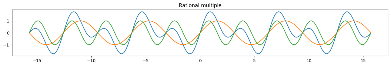
It is known that the sum of two periodic signals is itself periodic with a period that is equal to the least common multiple of the periods of the two summands, if and only if the two periods are rational multiples of each other. If the ratio of the two periods is irrational, then their sum will not be periodic itself.

Due to the floating-point representation in neural network libraries, this case cannot occur in practice, and all functions parameterized by Siren indeed have to be periodic.

Yet, the period of the resulting function may in practice be several orders of magnitudes larger than the period of each Siren neuron!

Let’s test this with two sines.

with torch.no_grad():
    coords = get_mgrid(210, 1) * 5 * np.pi
    
    sin_1 = torch.sin(coords)
    sin_2 = torch.sin(coords * 2)
    sum = sin_1 + sin_2
    
    fig, ax = plt.subplots(figsize=(16,2))
    ax.plot(coords, sum)
    ax.plot(coords, sin_1)
    ax.plot(coords, sin_2)
    plt.title("Rational multiple")
    plt.show()
    
    sin_1 = torch.sin(coords)
    sin_2 = torch.sin(coords * np.pi)
    sum = sin_1 + sin_2
    
    fig, ax = plt.subplots(figsize=(16,2))
    ax.plot(coords, sum)
    ax.plot(coords, sin_1)
    ax.plot(coords, sin_2)
    plt.title("Pseudo-irrational multiple")
    plt.show()

png

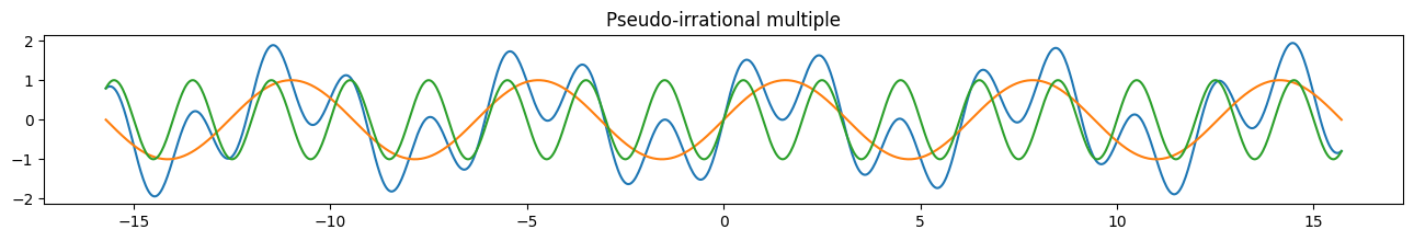
Though the second plot looks periodic, closer inspection shows that the period of the blue line is indeed larger than the range we’re sampling here.

Let’s take a look at what the Siren we just trained looks like outside its training domain!

with torch.no_grad():
    out_of_range_coords = get_mgrid(1024, 2) * 50
    model_out, _ = img_siren(out_of_range_coords.cuda())
    
    fig, ax = plt.subplots(figsize=(16,16))
    ax.imshow(model_out.cpu().view(1024,1024).numpy())
    plt.show()

png

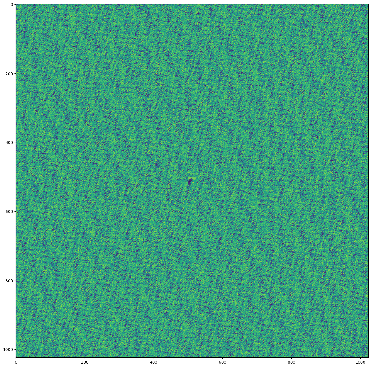
Though there is some self-similarity, the signal is not repeated on this range of (-50, 50).

Fitting an audio signal#

Here, we’ll use Siren to parameterize an audio signal - i.e., we seek to parameterize an audio waverform $f(t)$ at time points $t$ by a SIREN $\Phi$.

That is we seek the function $\Phi$ such that: $\mathcal{L}\int_\Omega \lVert \Phi(t) - f(t) \rVert \mathrm{d}t$ is minimized, in which $\Omega$ is the domain of the waveform.

For the audio, we’ll use the bach sonata:

import scipy.io.wavfile as wavfile
import io
from IPython.display import Audio

if not os.path.exists('gt_bach.wav'):
    !wget https://vsitzmann.github.io/siren/img/audio/gt_bach.wav

--2025-04-20 17:00:51--  https://vsitzmann.github.io/siren/img/audio/gt_bach.wav
Resolving vsitzmann.github.io (vsitzmann.github.io)... 185.199.110.153, 185.199.111.153, 185.199.108.153, ...
Connecting to vsitzmann.github.io (vsitzmann.github.io)|185.199.110.153|:443... connected.
HTTP request sent, awaiting response... 301 Moved Permanently
Location: https://www.vincentsitzmann.com/siren/img/audio/gt_bach.wav [following]
--2025-04-20 17:00:52--  https://www.vincentsitzmann.com/siren/img/audio/gt_bach.wav
Resolving www.vincentsitzmann.com (www.vincentsitzmann.com)... 185.199.108.153, 185.199.110.153, 185.199.109.153, ...
Connecting to www.vincentsitzmann.com (www.vincentsitzmann.com)|185.199.108.153|:443... connected.
HTTP request sent, awaiting response... 200 OK
Length: 1232886 (1.2M) [audio/wav]
Saving to: ‘gt_bach.wav’

gt_bach.wav         100%[===================>]   1.17M  25.5KB/s    in 49s     

2025-04-20 17:01:43 (24.7 KB/s) - ‘gt_bach.wav’ saved [1232886/1232886]

Let’s build a little dataset that computes coordinates for audio files:

class AudioFile(torch.utils.data.Dataset):
    def __init__(self, filename):
        self.rate, self.data = wavfile.read(filename)
        self.data = self.data.astype(np.float32)
        self.timepoints = get_mgrid(len(self.data), 1)

    def get_num_samples(self):
        return self.timepoints.shape[0]

    def __len__(self):
        return 1

    def __getitem__(self, idx):
        amplitude = self.data
        scale = np.max(np.abs(amplitude))
        amplitude = (amplitude / scale)
        amplitude = torch.Tensor(amplitude).view(-1, 1)
        return self.timepoints, amplitude

Let’s instantiate the Siren. As this audio signal has a much higer spatial frequency on the range of -1 to 1, we increase the $\omega_0$ in the first layer of siren.

bach_audio = AudioFile('gt_bach.wav')

dataloader = DataLoader(bach_audio, shuffle=True, batch_size=1, pin_memory=True, num_workers=0)

# Note that we increase the frequency of the first layer to match the higher frequencies of the
# audio signal. Equivalently, we could also increase the range of the input coordinates.
audio_siren = Siren(in_features=1, out_features=1, hidden_features=256, 
                    hidden_layers=3, first_omega_0=3000, outermost_linear=True)
audio_siren.cuda()

Siren(
  (net): Sequential(
    (0): SineLayer(
      (linear): Linear(in_features=1, out_features=256, bias=True)
    )
    (1): SineLayer(
      (linear): Linear(in_features=256, out_features=256, bias=True)
    )
    (2): SineLayer(
      (linear): Linear(in_features=256, out_features=256, bias=True)
    )
    (3): SineLayer(
      (linear): Linear(in_features=256, out_features=256, bias=True)
    )
    (4): Linear(in_features=256, out_features=1, bias=True)
  )
)

Let’s have a quick listen to ground truth:

rate, _ = wavfile.read('gt_bach.wav')

model_input, ground_truth = next(iter(dataloader))
Audio(ground_truth.squeeze().numpy(),rate=rate)

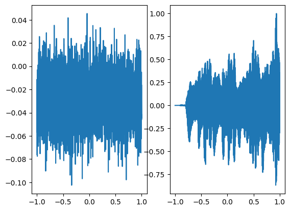
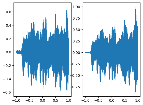
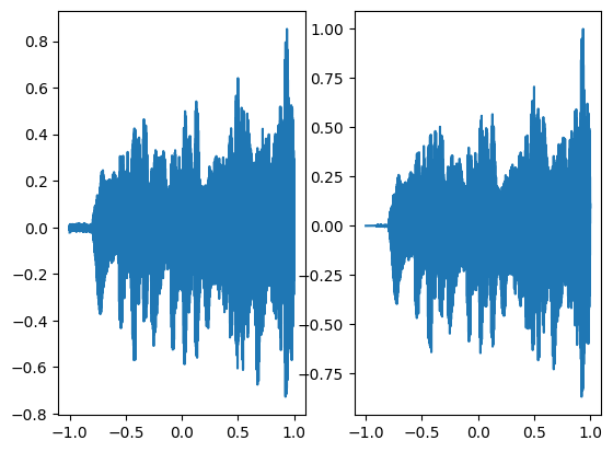
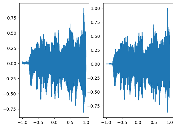
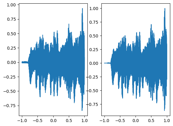
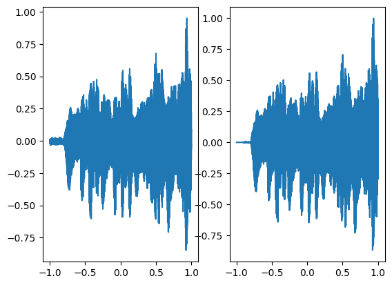
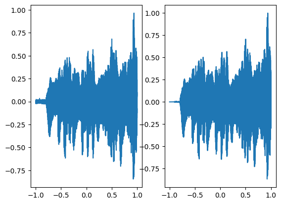
We now fit the Siren to this signal.

total_steps = 1000 
steps_til_summary = 100

optim = torch.optim.Adam(lr=1e-4, params=audio_siren.parameters())

model_input, ground_truth = next(iter(dataloader))
model_input, ground_truth = model_input.cuda(), ground_truth.cuda()

for step in range(total_steps):
    model_output, coords = audio_siren(model_input)    
    loss = F.mse_loss(model_output, ground_truth)
    
    if not step % steps_til_summary:
        print("Step %d, Total loss %0.6f" % (step, loss))
    
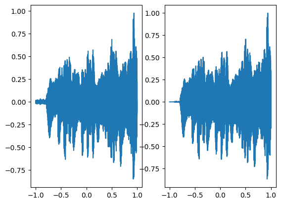
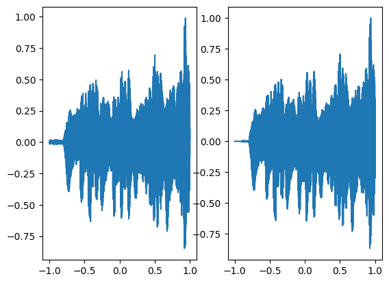
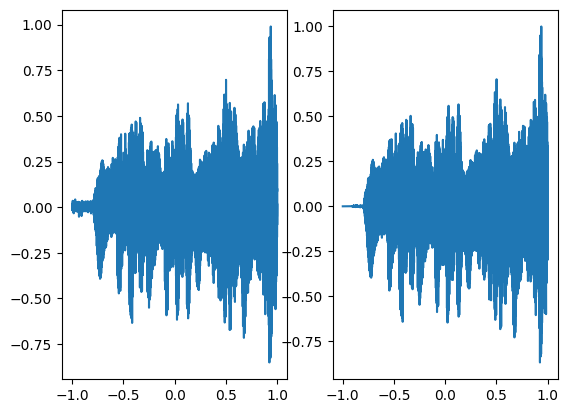
        fig, axes = plt.subplots(1,2)
        axes[0].plot(coords.squeeze().detach().cpu().numpy(),model_output.squeeze().detach().cpu().numpy())
        axes[1].plot(coords.squeeze().detach().cpu().numpy(),ground_truth.squeeze().detach().cpu().numpy())
        plt.show()

    optim.zero_grad()
    loss.backward()
    optim.step()

Step 0, Total loss 0.025330

png

Step 100, Total loss 0.003217

png

Step 200, Total loss 0.001231

png

Step 300, Total loss 0.001289

png

Step 400, Total loss 0.000717

png

Step 500, Total loss 0.000654

png

Step 600, Total loss 0.000469

png

Step 700, Total loss 0.000492

png

Step 800, Total loss 0.000264

png

Step 900, Total loss 0.000193

png

final_model_output, coords = audio_siren(model_input)
Audio(final_model_output.cpu().detach().squeeze().numpy(),rate=rate)

As we can see, within few iterations, Siren has approximated the audio signal very well!

Solving Poisson’s equation#

Now, let’s make it a bit harder. Let’s say we want to reconstruct an image but we only have access to its gradients!

That is, we now seek the function $\Phi$ such that: $\mathcal{L}=\int_{\Omega} \lVert \nabla\Phi(\mathbf{x}) - \nabla f(\mathbf{x}) \rVert\mathrm{d}\mathbf{x}$ is minimized, in which $\Omega$ is the domain of the image.

import scipy.ndimage
    
class PoissonEqn(Dataset):
    def __init__(self, sidelength):
        super().__init__()
        img = get_cameraman_tensor(sidelength)
        
        # Compute gradient and laplacian       
        grads_x = scipy.ndimage.sobel(img.numpy(), axis=1).squeeze(0)[..., None]
        grads_y = scipy.ndimage.sobel(img.numpy(), axis=2).squeeze(0)[..., None]
        grads_x, grads_y = torch.from_numpy(grads_x), torch.from_numpy(grads_y)
                
        self.grads = torch.stack((grads_x, grads_y), dim=-1).view(-1, 2)
        self.laplace = scipy.ndimage.laplace(img.numpy()).squeeze(0)[..., None]
        self.laplace = torch.from_numpy(self.laplace)
        
        self.pixels = img.permute(1, 2, 0).view(-1, 1)
        self.coords = get_mgrid(sidelength, 2)

    def __len__(self):
        return 1

    def __getitem__(self, idx):
        return self.coords, {'pixels':self.pixels, 'grads':self.grads, 'laplace':self.laplace}

Instantiate SIREN model#

cameraman_poisson = PoissonEqn(128)
dataloader = DataLoader(cameraman_poisson, batch_size=1, pin_memory=True, num_workers=0)

poisson_siren = Siren(in_features=2, out_features=1, hidden_features=256, 
                      hidden_layers=3, outermost_linear=True)
poisson_siren.cuda()

Siren(
  (net): Sequential(
    (0): SineLayer(
      (linear): Linear(in_features=2, out_features=256, bias=True)
    )
    (1): SineLayer(
      (linear): Linear(in_features=256, out_features=256, bias=True)
    )
    (2): SineLayer(
      (linear): Linear(in_features=256, out_features=256, bias=True)
    )
    (3): SineLayer(
      (linear): Linear(in_features=256, out_features=256, bias=True)
    )
    (4): Linear(in_features=256, out_features=1, bias=True)
  )
)

Define the loss function#

def gradients_mse(model_output, coords, gt_gradients):
    # compute gradients on the model
    gradients = gradient(model_output, coords)
    # compare them with the ground-truth
    gradients_loss = torch.mean((gradients - gt_gradients).pow(2).sum(-1))
    return gradients_loss

Train the model#

total_steps = 1000
steps_til_summary = 10

optim = torch.optim.Adam(lr=1e-4, params=poisson_siren.parameters())

model_input, gt = next(iter(dataloader))
gt = {key: value.cuda() for key, value in gt.items()}
model_input = model_input.cuda()

for step in range(total_steps):
    start_time = time.time()

    model_output, coords = poisson_siren(model_input)
    train_loss = gradients_mse(model_output, coords, gt['grads'])

    if not step % steps_til_summary:
        print("Step %d, Total loss %0.6f, iteration time %0.6f" % (step, train_loss, time.time() - start_time))

        img_grad = gradient(model_output, coords)
        img_laplacian = laplace(model_output, coords)

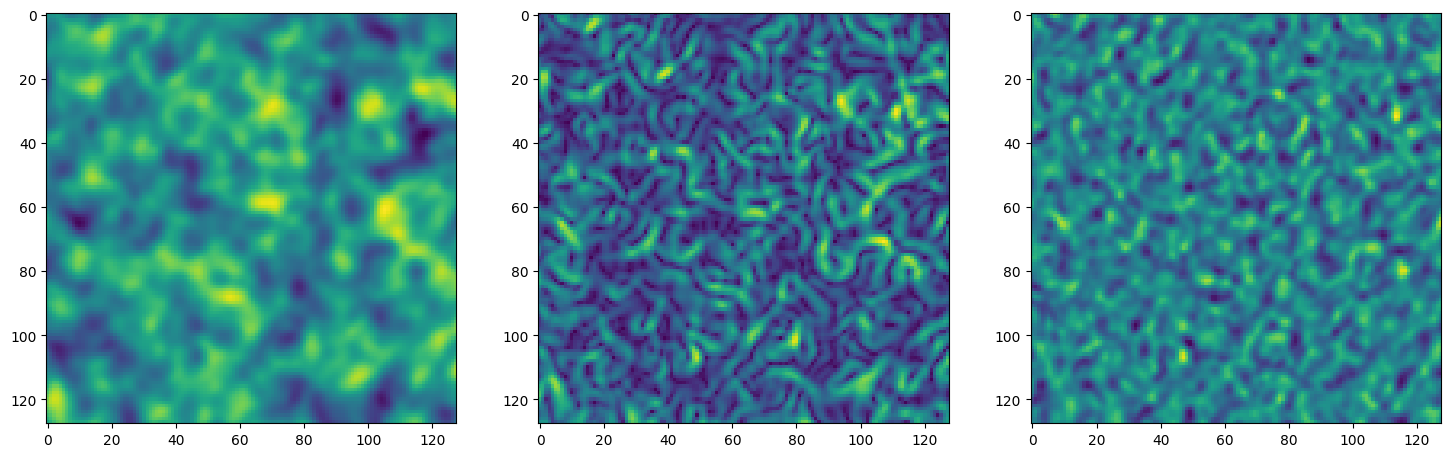
        fig, axes = plt.subplots(1, 3, figsize=(18, 6))
        axes[0].imshow(model_output.cpu().view(128,128).detach().numpy())
        axes[1].imshow(img_grad.cpu().norm(dim=-1).view(128,128).detach().numpy())
        axes[2].imshow(img_laplacian.cpu().view(128,128).detach().numpy())
        plt.show()
        
    optim.zero_grad()
    train_loss.backward()
    optim.step()

Step 0, Total loss 16.082405, iteration time 0.003057

png

Step 10, Total loss 4.434361, iteration time 0.001914

png

Step 20, Total loss 1.665594, iteration time 0.001487

png

Step 30, Total loss 0.724829, iteration time 0.001626

png

Step 40, Total loss 0.335272, iteration time 0.001631

png

Step 50, Total loss 0.184486, iteration time 0.001456

png

Step 60, Total loss 0.123615, iteration time 0.001555

png

Step 70, Total loss 0.092790, iteration time 0.001478

png

Step 80, Total loss 0.071172, iteration time 0.001442

png

Step 90, Total loss 0.059844, iteration time 0.001549

png

Step 100, Total loss 0.051608, iteration time 0.001558

png

Step 110, Total loss 0.047639, iteration time 0.001494

png

Step 120, Total loss 0.070216, iteration time 0.001613

png

Step 130, Total loss 0.042079, iteration time 0.001813

png

Step 140, Total loss 0.038912, iteration time 0.001719

png

Step 150, Total loss 0.033385, iteration time 0.001613

png

Step 160, Total loss 0.030420, iteration time 0.001530

png

Step 170, Total loss 0.028471, iteration time 0.001814

png

Step 180, Total loss 0.038084, iteration time 0.001581

png

Step 190, Total loss 0.029641, iteration time 0.001464

png

Step 200, Total loss 0.025058, iteration time 0.001628

png

Step 210, Total loss 0.023223, iteration time 0.001459

png

Step 220, Total loss 0.022123, iteration time 0.001582

png

Step 230, Total loss 0.036758, iteration time 0.001497

png

Step 240, Total loss 0.021620, iteration time 0.001488

png

Step 250, Total loss 0.020993, iteration time 0.001635

png

Step 260, Total loss 0.019381, iteration time 0.001593

png

Step 270, Total loss 0.020076, iteration time 0.001535

png

Step 280, Total loss 0.030141, iteration time 0.001494

png

Step 290, Total loss 0.018392, iteration time 0.001555

png

Step 300, Total loss 0.016569, iteration time 0.001529

png

Step 310, Total loss 0.016443, iteration time 0.001474

png

Step 320, Total loss 0.015786, iteration time 0.001573

png

Step 330, Total loss 0.039000, iteration time 0.001455

png

Step 340, Total loss 0.022057, iteration time 0.001545

png

Step 350, Total loss 0.016721, iteration time 0.001589

png

Step 360, Total loss 0.014248, iteration time 0.001584

png

Step 370, Total loss 0.013907, iteration time 0.001489

png

Step 380, Total loss 0.013540, iteration time 0.001573

png

Step 390, Total loss 0.014559, iteration time 0.001492

png

Step 400, Total loss 0.017451, iteration time 0.001518

png

Step 410, Total loss 0.014687, iteration time 0.001617

png

Step 420, Total loss 0.012690, iteration time 0.001566

png

Step 430, Total loss 0.012461, iteration time 0.001595

png

Step 440, Total loss 0.011988, iteration time 0.001545

png

Step 450, Total loss 0.011807, iteration time 0.001588

png

Step 460, Total loss 0.013722, iteration time 0.001428

png

Step 470, Total loss 0.022628, iteration time 0.001519

png

Step 480, Total loss 0.016508, iteration time 0.001616

png

Step 490, Total loss 0.012050, iteration time 0.001658

png

Step 500, Total loss 0.011336, iteration time 0.001584

png

Step 510, Total loss 0.010884, iteration time 0.001501

png

Step 520, Total loss 0.010552, iteration time 0.001600

png

Step 530, Total loss 0.010350, iteration time 0.001571

png

Step 540, Total loss 0.010176, iteration time 0.001546

png

Step 550, Total loss 0.010027, iteration time 0.001560

png

Step 560, Total loss 0.010373, iteration time 0.001611

png

Step 570, Total loss 0.044359, iteration time 0.001496

png

Step 580, Total loss 0.016315, iteration time 0.001571

png

Step 590, Total loss 0.011208, iteration time 0.001516

png

Step 600, Total loss 0.010159, iteration time 0.001469

png

Step 610, Total loss 0.009454, iteration time 0.001600

png

Step 620, Total loss 0.009159, iteration time 0.001560

png

Step 630, Total loss 0.008941, iteration time 0.001639

png

Step 640, Total loss 0.008817, iteration time 0.001563

png

Step 650, Total loss 0.008752, iteration time 0.001638

png

Step 660, Total loss 0.023890, iteration time 0.001548

png

Step 670, Total loss 0.011903, iteration time 0.001833

png

Step 680, Total loss 0.010384, iteration time 0.001573

png

Step 690, Total loss 0.008881, iteration time 0.001731

png

Step 700, Total loss 0.008381, iteration time 0.001497

png

Step 710, Total loss 0.008077, iteration time 0.001451

png

Step 720, Total loss 0.007929, iteration time 0.001637

png

Step 730, Total loss 0.007788, iteration time 0.001428

png

Step 740, Total loss 0.007790, iteration time 0.001869

png

Step 750, Total loss 0.023985, iteration time 0.001502

png

Step 760, Total loss 0.014367, iteration time 0.001581

png

Step 770, Total loss 0.009977, iteration time 0.001491

png

Step 780, Total loss 0.008088, iteration time 0.001537

png

Step 790, Total loss 0.007420, iteration time 0.001494

png

Step 800, Total loss 0.007165, iteration time 0.001528

png

Step 810, Total loss 0.006995, iteration time 0.001772

png

Step 820, Total loss 0.006945, iteration time 0.001549

png

Step 830, Total loss 0.010760, iteration time 0.001468

png

Step 840, Total loss 0.009743, iteration time 0.001571

png

Step 850, Total loss 0.007500, iteration time 0.001482

png

Step 860, Total loss 0.006997, iteration time 0.001571

png

Step 870, Total loss 0.006662, iteration time 0.001717

png

Step 880, Total loss 0.006393, iteration time 0.002085

png

Step 890, Total loss 0.006251, iteration time 0.001374

png

Step 900, Total loss 0.006207, iteration time 0.001548

png

Step 910, Total loss 0.012152, iteration time 0.001693

png

Step 920, Total loss 0.015004, iteration time 0.001559

png

Step 930, Total loss 0.008816, iteration time 0.001462

png

Step 940, Total loss 0.006670, iteration time 0.001614

png

Step 950, Total loss 0.006041, iteration time 0.001507

png

Step 960, Total loss 0.005791, iteration time 0.001564

png

Step 970, Total loss 0.005623, iteration time 0.001581

png

Step 980, Total loss 0.005517, iteration time 0.001659

png

Step 990, Total loss 0.005425, iteration time 0.001589

png

Initialization scheme & distribution of activations#

We now reproduce the empirical result on the distribution of activations, and will thereafter show empirically that the distribution of activations is shift-invariant as well!

from collections import OrderedDict
import matplotlib
import numpy.fft as fft
import scipy.stats as stats


def eformat(f, prec, exp_digits):
    s = "%.*e"%(prec, f)
    mantissa, exp = s.split('e')
    # add 1 to digits as 1 is taken by sign +/-
    return "%se%+0*d"%(mantissa, exp_digits+1, int(exp))

def format_x_ticks(x, pos):
    """Format odd tick positions
    """
    return eformat(x, 0, 1)

def format_y_ticks(x, pos):
    """Format odd tick positions
    """
    return eformat(x, 0, 1)

def get_spectrum(activations):
    n = activations.shape[0]

    spectrum = fft.fft(activations.numpy().astype(np.double).sum(axis=-1), axis=0)[:n//2]
    spectrum = np.abs(spectrum)

    max_freq = 100                
    freq = fft.fftfreq(n, 2./n)[:n//2]
    return freq[:max_freq], spectrum[:max_freq]


def plot_all_activations_and_grads(activations):
    num_cols = 4
    num_rows = len(activations)
    
    fig_width = 5.5
    fig_height = num_rows/num_cols*fig_width
    fig_height = 9
    
    fontsize = 5
        
    fig, axs = plt.subplots(num_rows, num_cols, gridspec_kw={'hspace': 0.3, 'wspace': 0.2},
                            figsize=(fig_width, fig_height), dpi=300)
    
    axs[0][0].set_title("Activation Distribution", fontsize=7, fontfamily='serif', pad=5.)
    axs[0][1].set_title("Activation Spectrum", fontsize=7, fontfamily='serif', pad=5.)
    axs[0][2].set_title("Gradient Distribution", fontsize=7, fontfamily='serif', pad=5.)
    axs[0][3].set_title("Gradient Spectrum", fontsize=7, fontfamily='serif', pad=5.)

    x_formatter = matplotlib.ticker.FuncFormatter(format_x_ticks)
    y_formatter = matplotlib.ticker.FuncFormatter(format_y_ticks)

    spec_rows = []
    for idx, (key, value) in enumerate(activations.items()):    
        grad_value = value.grad.cpu().detach().squeeze(0)
        flat_grad = grad_value.view(-1)
        axs[idx][2].hist(flat_grad, bins=256, density=True)
        
        value = value.cpu().detach().squeeze(0) # (1, num_points, 256)
        n = value.shape[0]
        flat_value = value.view(-1)
            
        axs[idx][0].hist(flat_value, bins=256, density=True)
                
        if idx>1:
            if not (idx)%2:
                x = np.linspace(-1, 1., 500)
                axs[idx][0].plot(x, stats.arcsine.pdf(x, -1, 2), 
                                 linestyle=':', markersize=0.4, zorder=2)
            else:
                mu = 0
                variance = 1
                sigma = np.sqrt(variance)
                x = np.linspace(mu - 3*sigma, mu + 3*sigma, 500)
                axs[idx][0].plot(x, stats.norm.pdf(x, mu, sigma), 
                                 linestyle=':', markersize=0.4, zorder=2)
        
        activ_freq, activ_spec = get_spectrum(value)
        axs[idx][1].plot(activ_freq, activ_spec)
        
        grad_freq, grad_spec = get_spectrum(grad_value)
        axs[idx][-1].plot(grad_freq, grad_spec)
        
        for ax in axs[idx]:
            ax.tick_params(axis='both', which='major', direction='in',
                                    labelsize=fontsize, pad=1., zorder=10) 
            ax.tick_params(axis='x', labelrotation=0, pad=1.5, zorder=10) 

            ax.xaxis.set_major_formatter(x_formatter)
            ax.yaxis.set_major_formatter(y_formatter)

model = Siren(in_features=1, hidden_features=2048, 
              hidden_layers=10, out_features=1, outermost_linear=True)

input_signal = torch.linspace(-1, 1, 65536//4).view(1, 65536//4, 1)
activations = model.forward_with_activations(input_signal, retain_grad=True)
output = activations[next(reversed(activations))]

# Compute gradients. Because we have retain_grad=True on 
# activations, each activation stores its own gradient!
output.mean().backward()

plot_all_activations_and_grads(activations)

png

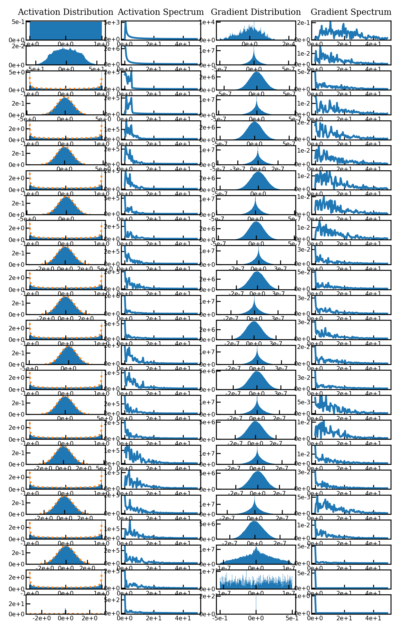
Note how the activations of Siren always alternate between a standard normal distribution with standard deviation one, and an arcsine distribution. If you have a beefy computer, you can put this to the extreme and increase the number of layers - this property holds even for more than 50 layers!

Distribution of activations is shift-invariant#

One of the key properties of the periodic sine nonlinearity is that it affords a degree of shift-invariance. Consider the first layer of a Siren: You can convince yourself that this layer can easily learn to map two different coordinates to the same set of activations. This means that whatever layers come afterwards will apply the same function to these two sets of coordinates.

Moreoever, the distribution of activations similarly are shift-invariant. Let’s shift our input signal by 1000 and re-compute the activations:

input_signal = torch.linspace(-1, 1, 65536//4).view(1, 65536//4, 1) + 1000
activations = model.forward_with_activations(input_signal, retain_grad=True)
output = activations[next(reversed(activations))]

# Compute gradients. Because we have retain_grad=True on 
# activations, each activation stores its own gradient!
output.mean().backward()

plot_all_activations_and_grads(activations)

png

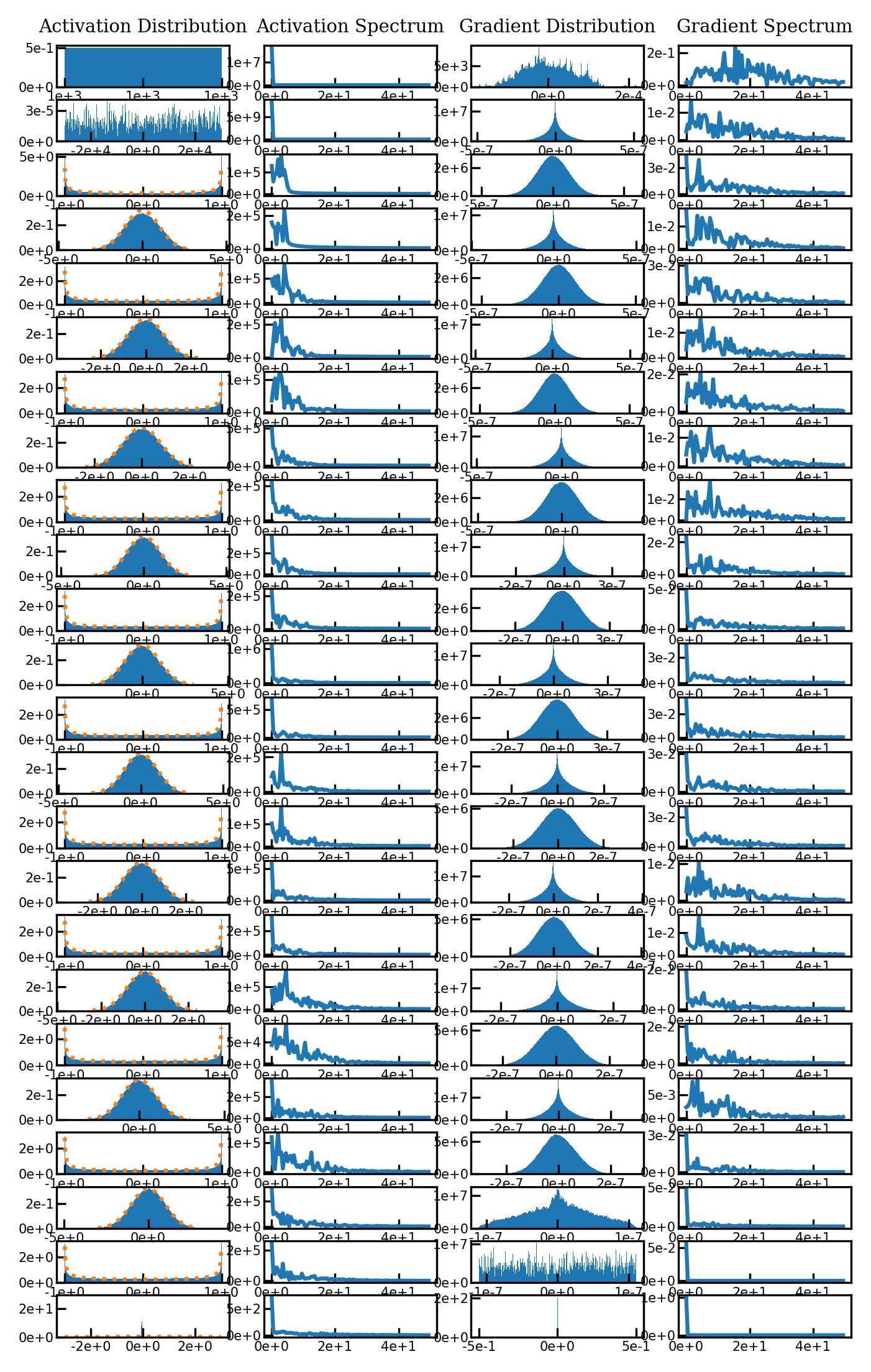
As we can see, the distributions of activations didn’t change at all - they are perfectly invariant to the shift.